In AI engineering, we work with high-dimensional data every day. Whether it’s embeddings, input features, weights, or gradients, they are all vectors. Mastering vector operations like addition, subtraction, multiplication, and division is essential to building efficient AI systems.
What Is a Vector?
Before we proceed, let’s briefly remind ourselves about vectors. In mathematics, vectors are entities characterized by magnitude and direction. In NumPy, vectors are represented using arrays, which are more efficient than standard Python lists for numerical operations. Here’s how you would represent a vector in NumPy:
|
1 2 3 |
import numpy as np vector_example = np.array([1, 2, 3]) |
In this example, np.array([1, 2, 3]) creates a vector with values 1, 2, and 3. NumPy arrays provide powerful capabilities to perform mathematical operations efficiently, which we’ll explore in this lesson.
1. Vector Operation – Addition
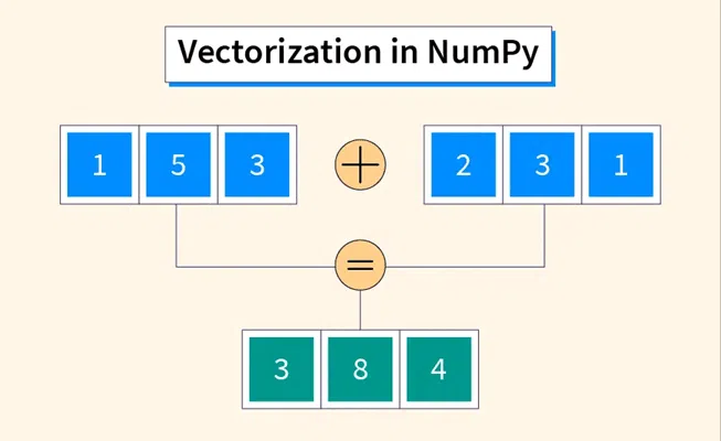
To add two vectors in NumPy, you can use the np.add() function or simply use Python’s addition operator +. Here’s an example using np.add(): Formula:
|
1 |
A + B = [a₁ + b₁, a₂ + b₂, ..., an + bn] |
Example (Python):
|
1 2 3 4 5 6 7 8 9 10 |
import numpy as np vector_a = np.array([1, 2, 3]) vector_b = np.array([4, 5, 6]) addition = np.add(vector_a, vector_b) print("Addition:", addition) # Output: # Addition: [5 7 9] |
In this example, each element of vector_a is added to the corresponding element of vector_b, resulting in a new vector [5, 7, 9].
2. Vector Operation – Subtraction
Similar to addition, vector subtraction can be performed with np.subtract() or the subtraction operator -. Here’s how: Formula:
|
1 |
A - B = [a₁ - b₁, a₂ - b₂, ..., an - bn] |
Example:
|
1 2 3 4 5 |
subtraction = np.subtract(vector_a, vector_b) print("Subtraction:", subtraction) # Output: # Subtraction: [-3 -3 -3] |
This example subtracts each element of vector_b from the corresponding element of vector_a, resulting in [-3, -3, -3]. Note that for both the subtraction and addition operations, they are performed only if the dimensions (shape) of the vectors are equal. This ensures that corresponding elements are properly aligned for these operations.
3. Scalar Multiplication
Scalar multiplication involves multiplying each element of a vector by a scalar value. Here’s an example with NumPy:
|
1 2 3 4 5 |
scalar_multiplication = 2 * vector_a print("Scalar Multiplication (2 * A):", scalar_multiplication) # Output: # Scalar Multiplication (2 * A): [2 4 6] |
In this case, each element of vector_a is multiplied by the scalar 2, yielding [2, 4, 6].
4. Calculating Dot Product
The dot product is a mathematical operation that takes two vectors and combines them to produce a single scalar value. This scalar value is a measure of how well-aligned the two vectors are in terms of direction. Mathematically, the dot product of two vectors is the sum of the products of their corresponding components. It is a crucial operation in determining the angle between vectors, as well as in finding projections.
|
1 2 3 4 5 6 7 8 9 10 11 12 13 14 15 16 17 18 19 20 21 |
import numpy as np # Defining vectors vector_a = np.array([1, 2, 3]) vector_b = np.array([4, 5, 6]) # Dot product using np.dot and @ operator dot_product = np.dot(vector_a, vector_b) dot_product_alt = vector_a @ vector_b # Display results print("Vector A:", vector_a) print("Vector B:", vector_b) print("Dot Product (np.dot):", dot_product) print("Dot Product (@ operator):", dot_product_alt) # Output: # Vector A: [1 2 3] # Vector B: [4 5 6] # Dot Product (np.dot): 32 # Dot Product (@ operator): 32 |
- We start by defining two vectors,
vector_aandvector_b, usingNumPyarrays. - The dot product is computed using both
np.dot(vector_a, vector_b)andvector_a @ vector_b, demonstratingNumPy‘s flexibility in syntax. - The result, a scalar, is printed out, indicating the degree of alignment between the vectors.
Here, the dot product of the two vectors is 32, showing their level of alignment.
4. Calculating Cross Product
Now, let’s explore the cross product, a fundamental vector operation in 3D space. The cross product of two vectors results in a third vector that is perpendicular to both of the original vectors, making it highly valuable in applications such as determining rotational forces and calculating normal vectors on surfaces. The magnitude of the cross product vector is proportional to the area of the parallelogram formed by the two initial vectors, providing a geometric interpretation of the operation.
|
1 2 3 4 5 6 7 8 9 10 11 12 13 14 15 16 17 18 |
import numpy as np # Defining vectors vector_a = np.array([1, 2, 3]) vector_b = np.array([4, 5, 6]) # Cross product cross_product = np.cross(vector_a, vector_b) # Display results print("Vector A:", vector_a) print("Vector B:", vector_b) print("Cross Product:", cross_product) # Output: # Vector A: [1 2 3] # Vector B: [4 5 6] # Cross Product: [-3 6 -3] |
- We define the same vectors,
vector_aandvector_b. - The cross product is calculated using
np.cross(vector_a, vector_b). - The result is a vector that is perpendicular to both
vector_aandvector_b.
The output vector [-3, 6, -3] is orthogonal to both input vectors.
5. Vector Operation – Multiplication
Vector multiplication comes in two common forms:
i) Element-wise Multiplication (Hadamard Product)
|
1 |
A * B = [a₁ * b₁, a₂ * b₂, ..., aₙ * bₙ] |
|
1 2 |
print("Element-wise Multiplication:", a * b) # Output: [2 12 30] |
ii) Dot Product (Inner Product)
|
1 |
A · B = a₁×b₁ + a₂×b₂ + ... + an×bn |
|
1 2 3 |
dot = np.dot(a, b) print("Dot Product:", dot) # Output: 44 |
6. Vector Operation – Division
There is no defined “dot division,” but element-wise division is commonly used.
Formula:
|
1 |
A / B = [a₁ / b₁, a₂ / b₂, ..., an / bn] |
Example:
|
1 2 |
print("Element-wise Division:", a / b) # Output: [2. 1.3333 1.2] |
N.B: Always handle division by zero appropriately.
Summary Table
| Operation | Formula | Common AI Applications |
|---|---|---|
| Addition | [a₁ + b₁, …, aₙ + bₙ] | Semantic composition, gradients |
| Subtraction | [a₁ – b₁, …, aₙ – bₙ] | Distance, feature differences |
| Multiplication | Dot or Element-wise | Similarly, attention, gating |
| Division | [a₁ / b₁, …, aₙ / bₙ] | Normalization, scaling |
From NLP and computer vision to optimization, vector operations are foundational in AI. The better you understand these operations, the more confidently you’ll be able to design, debug, and optimize AI models.


Leave a Comment