In this article, we'll take a look at
Show
5. UNSUPERVISED LEARNING ALGORITHMS
Unsupervised learning finds hidden patterns in unlabeled data. Unlike supervised learning, it doesn’t rely on labeled outputs (no predefined target).
5.1) K-Means Clustering
5.1.1) Algorithm Overview
K-Means is a clustering algorithm that divides data into K clusters based on similarity.
It works by:
It works by:
- Selecting K random centroids.
- Assigning each point to the nearest centroid.
- Updating the centroid to the mean of its assigned points.
- Repeat steps 2–3 until the centroids stop changing.
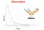
5.1.2) Elbow Method
- Used to choose the optimal number of clusters (K).
- Plot the number of clusters (K) vs. Within-Cluster-Sum-of-Squares (WCSS).
- The point where the WCSS curve bends (elbow) is the best K.
5.1.3) K-Means++ Initialization
- Improves basic K-Means by smartly selecting initial centroids, reducing the chance of poor clustering.
- Starts with one random centroid, then selects the next ones based on distance from the current ones (probabilistically).
5.2) Hierarchical Clustering
5.2.1) Agglomerative vs. Divisive Clustering
- Agglomerative (bottom-up): Start with each point as its own cluster and merge the closest clusters.
- Divisive (top-down): Start with one large cluster and recursively split it.
Agglomerative is more commonly used.
5.2.2) Dendrogram and Optimal Cut
- A dendrogram is a tree-like diagram that shows how clusters are formed at each step.
- The height of branches represents the distance between clusters.
- Cutting the dendrogram at a certain height gives the desired number of clusters.
5.3) Principal Component Analysis (PCA)
PCA is a dimensionality reduction technique used to simplify datasets while retaining most of the important information.
5.3.1) Dimensionality Reduction
- PCA transforms the data into a new coordinate system with fewer dimensions (called principal components).
- Useful for visualization, speeding up algorithms, and avoiding the curse of dimensionality.
5.3.2) Eigenvalue Decomposition
- PCA is based on eigenvectors and eigenvalues of the covariance matrix of the data.
- The eigenvectors define the new axes (principal components).
- The eigenvalues indicate the amount of variance each component captures.
5.3.3) Scree Plot and Explained Variance
- Scree Plot: A plot of eigenvalues to help decide how many components to keep.
- The explained variance ratio shows how much of the data’s variance is captured by each component.
5.4) DBSCAN (Density-Based Spatial Clustering of Applications with Noise)
DBSCAN is a density-based clustering algorithm that groups closely packed points and marks outliers as noise.
5.4.1) Density-Based Clustering
Unlike K-Means, DBSCAN doesn’t require specifying the number of clusters. Clusters are formed based on dense regions in the data.
5.4.2) Epsilon and MinPts Parameters
- Epsilon (ε): Radius around a point to search for neighbors.
- MinPts: Minimum number of points required to form a dense region.
- Points are classified as:
- Core Point: Has MinPts within ε.
- Border Point: Not a core but within ε of a core.
- Noise: Neither core nor border.


Leave a Comment